23  Tipos de gráficas

En esta sección del curso, exploraremos las técnicas visuales disponibles en Matplotlib para representar datos por pares, o Pairwise data.

Desde el gráfico de líneas hasta herramientas como fill_between y stackplot, descubriremos cómo cada tipo de gráfico nos brinda una perspectiva única sobre la relación entre dos variables cuantitativas.

import pandas as pd
import matplotlib.pyplot as plt
from dateutil.parser import parse

f = '../data/Cuernavaca_1dia_comas.csv'
cuerna = pd.read_csv(f,index_col=0,parse_dates=True)
cuerna.head()

	To	Ws	Wd	P	Ig	Ib	Id
tiempo
2012-01-01 00:00:00	19.3	0.0	26	87415	0	0	0
2012-01-01 01:00:00	18.6	0.0	26	87602	0	0	0
2012-01-01 02:00:00	17.9	0.0	30	87788	0	0	0
2012-01-01 03:00:00	17.3	0.0	30	87554	0	0	0
2012-01-01 04:00:00	16.6	0.0	27	87321	0	0	0

fig, ax = plt.subplots()

ax.plot(cuerna.To)
ax.set_title('plot')

Text(0.5, 1.0, 'plot')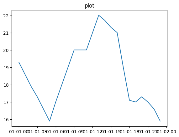

fig, ax =  plt.subplots()

ax.scatter(cuerna.index,cuerna.To)
ax.set_title('Scatter')

Text(0.5, 1.0, 'Scatter')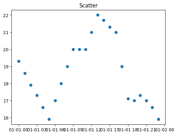

fig, ax = plt.subplots()
# f1 = parse("2012-01-01")
# f2 = f1 + pd.Timedelta("10H")

ax.bar(cuerna.index,cuerna.To)
# ax.bar(cuerna.index,cuerna.To,width=1/25)

ax.set_title('Bars')


# ax.set_xlim(f1,f2)

Text(0.5, 1.0, 'Bars')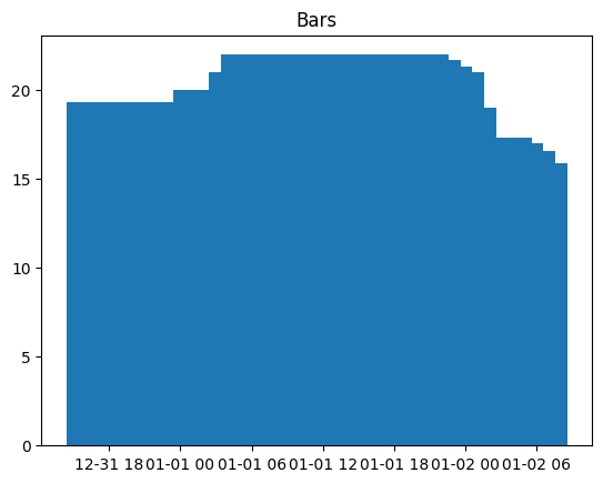

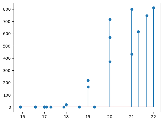
fig, ax = plt.subplots()

ax.stem(cuerna.To)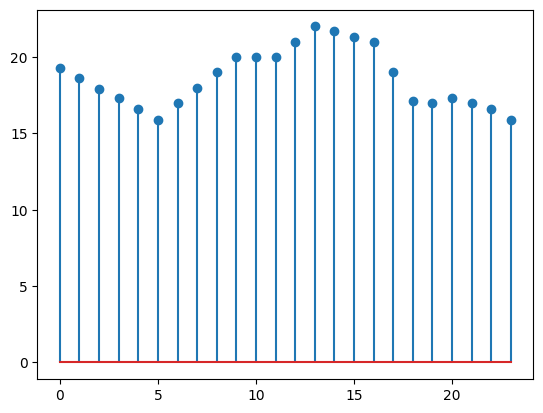

fig, ax = plt.subplots()

ax.fill_between(cuerna.index,cuerna.To.mean(),cuerna.To)
ax.plot(cuerna.To,'r-')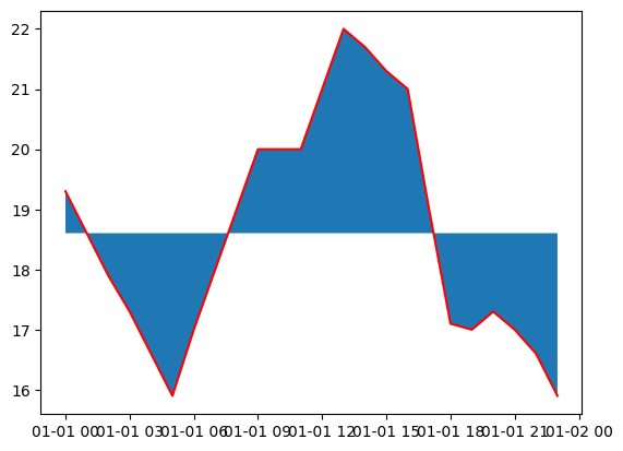

fig, ax = plt.subplots()

ax.stairs(cuerna.To)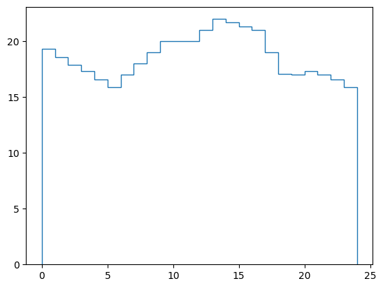

Por supuesto hay que escoger cada tipo de gr’afica de acuerdo a los datos y lo que queremos transmitir.

fig, ax = plt.subplots()

ax.scatter(cuerna.To, cuerna.Ig)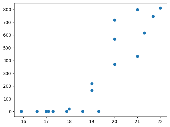

fig, ax = plt.subplots()

ax.stem(cuerna.To, cuerna.Ig)